* = forthcoming
Site navigation:
Contents
In the very clear dynamical systems and application-oriented setting of PyDSTool, we believe there is no inappropriate clash of terminology in naming the class Generator. The core of the Python language also contains a special class known as a generator, and we trust that no-one finds this confusing.
Generator objects compute multi-dimensional trajectories for the primary system state variables they define. Additional auxiliary variables may be specified that can be explicit functions of the system state. The values of auxiliary variables are also stored in the computed Trajectory object. The Trajectory class implements parameterized and non-parameterized trajectories and curves. Instantiated Trajectory objects that are parameterized are callable with independent variable values in a defined range. Trajectories are constructed by Generators, either explicitly or implicitly via a function, or by interpolating a mesh of points. When called like a function, Trajectory objects return a state value, using interpolation between mesh points if necessary. Currently only linear and quadratic interpolation is supported.
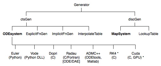
Generators come in two principal sub-classes, depending on the representation of the independent variable. This variable may either be represented in a continuous domain or a discrete domain. All Generator instances are sub-typed from one of these super classes, ctsGen or discGen. The most common Generators, of sub-classes ODEsystem and MapSystem, are for solving initial value problems (marked in bold in the chart below). There are presently no solvers for boundary value problems, although there are a few Python-based solvers available elsewhere The following chart shows the class hierarchy of Generator.
Depending on the type of Generator, the user may need to specify parameter values and initial conditions that uniquely determine the Trajectory that will be created when the Generator's compute method is called. Generators can contain a specification for events that can be detected during the computation of a trajectory. These events are specified as zero crossings of functions in the state variables or of the independent variable. Some forms of Generator also permit autonomous external inputs to be supplied in the form of a Trajectory object (see below).
After computation of a Trajectory, any errors or warnings produced during the computation are recorded in the Generator object's Diagnostics attribute, and can be queried or reset.
The "right-hand side" function specifications for Generators are not provided by hand-written code, which would be inconvenient and would burden the user with too much book-keeping with array indices, etc. Instead, the user specifies a dictionary of definitions for these functions, keyed by the variable names (see FunctionalSpec). In turn, these dictionaries can be created automatically using the ModelSpec and ModelConstructor class utilities for PyDSTool symbolic expressions, described elsewhere. The ModelSpec.Quantity classes can also be used in place of string definitions (see the example tests/Tutorial_SymbolicJac.py).
Preset sub-domains of the real numbers can be specified for each state variable, for the independent variable of the system ("time"), and for the parameters. These bounds can help with error checking and validation of a model, and can be crucial for setting up some types of hybrid system. The Generator initialization keys for these bounds are 'xdomain', 'tdomain', and 'pdomain', respectively.
The arguments to the Generator's initialization call can be made most easily by first assembling them in an argument structure. See the GettingStarted page for examples.
Uniformly sample the named trajectory over range indicated. Returns a Pointset. If doEvents=True (default), the event points for the trajectory are included in the output, regardless of the dt sampling rate. The order of variable names given in the 'coords' argument is ignored.
precise=True causes the trajectory position to be evaluated precisely at the t values specified, which will invoke slow interpolation (requires dt to be set otherwise an exception will be raised).
precise=False (default) causes the nearest underlying mesh positions to be used, if available (otherwise the behaviour is the same as precise=True provided dt has been set, otherwise an exception will be raised).
If dt is not given, the underlying time mesh is used, if available.
Return a dictionary of the underlying independent variables` meshes, where they exist. (Dictionary contains references to the meshes, not copies of the meshes.) Always returns data in local time frame.
[FScompat option selects whether to use FuncSpec compatible naming for variables (mainly for internal use).]
We may now introspect the 'traj' object to investigate its properties, using the object's info() method and the inbuilt function dir(). For attributes only, info() gives much more useful output than the basic inbuilt call to dir(), but does not indicate the object's available methods. Better still is to call print API(traj), but the output will be extensive!
>>> print traj.info(1) # i.e., verbose level 1
 Trajectory test of variables: ['y', 'w']
 over domains: {'y': Interval traj_dep_bd, 'w': Interval traj_dep_bd}
The 'indepdomain' attribute is an Interval object. The 'depdomain' attribute is a dictionary of Interval objects, one for each dependent variable.
>>> print traj.indepdomain.info()
Interval traj_indep_bd
  float: traj_indep_bd = [0,10.0] @ eps = 1e-014
>>> print testtraj.depdomain['w'].info()
Interval traj_dep_bd
  float: traj_dep_bd = [30.0,315.701094773] @ eps = 1e-014
The @ eps = 1e-14 information is not usually significant to casual users. It denotes the error tolerance with which interval endpoints are resolved, when issues of arithmetic precision impede on the comparison of interval endpoints. Now, we look turning the Trajectory object into a form that can be displayed in a plot. We use the sample() method of the trajectory to extract values at a desired resolution. The result of this call is a Pointset object (which is essentially a context-laden and index-free array of time and variable values). For more details of this, see the Tutorial.
pts = traj.sample(dt=0.1) # Pointset sampled at intervals of 0.1
Utility function to convert one or more numeric type to a Trajectory. Option to make the trajectory parameterized or not, by pasing an indepvar value. To use integer types for trajectory coordinates unset the default all_types_float=True argument. To create interpolated (continuously defined) trajectories, set discrete=False, otherwise leave at its default value of True.
Convert a pointset into a trajectory using linear interpolation, retaining parameterization by an independent variable if present.
Attributes (followed by description and type)
The basic query keys always available are:
'pars' or 'parameters', 'events', 'abseps',
'ics' or 'initialconditions', 'vars' or 'variables',
'auxvariables' or 'auxvars', 'vardomains', 'pardomains'
The variables attribute will include any auxiliary variables. These may be used for monitoring functions of the variables (e.g. for plotting purposes), or they may be true variables of the system that are defined as algebraic functions of the dynamic variables.
Methods
The major methods for Generators are:
For Generators that support events (most of them), there are special set methods for control event parameters.
Each of these methods takes an event name and a new value as arguments
For many types of Generator, especially MapSystem and ODEsystem types (for initial value problems), other special methods are now discussed.
The RHS vector field function, any Jacobians, auxiliary variables, and all user-defined auxiliary functions are exposed to the user of the generator as python functions, and are called using the same calling sequence as they were defined. For a generator g, these are respectively defined as the methods Rhs, Jacobian, JacobianP (for Jac with respect to parameters), AuxVars, and auxfns.<aux_func_name>. Internal references to parameter names are mapped dynamically to the current values of the parameters in the generator's pars dictionary. If external inputs are defined then the system is non-autonomous, and the first 't' argument is used to fetch a value of the inputs internally to these methods.
Each Generator contains a Diagnostics object which can report errors and warnings found during a Trajectory computation. For a generator g, after such a computation you may call g.diagnostics.showWarnings() or g.diagnostics.showErrors() and to see information printed to the terminal. Alternatively, string versions can be returned from the 'getWarnings' and 'getErrors' methods. Any logged entries are cleared when the 'compute' method is next called. Codes and accompanying logged data correspond to information the following table:
errmessages = {E_NONUNIQUETERM: 'More than one terminal event found',
               E_COMPUTFAIL: 'Computation of trajectory failed'}

errorfields = {E_NONUNIQUETERM: ['t', 'event list'],
               E_COMPUTFAIL: ['t', 'error info']}

warnmessages = {W_UNCERTVAL: 'Uncertain value computed',
                W_TERMEVENT: 'Terminal event(s) found',
                W_NONTERMEVENT: 'Non-terminal event(s) found',
                W_TERMSTATEBD: 'State variable reached bounds (terminal)',
                W_BISECTLIMIT: 'Bisection limit reached for event',
                W_NONTERMSTATEBD: 'State or input variable reached bounds (non-terminal)'}

warnfields = {W_UNCERTVAL: ['value', 'interval'],
              W_TERMEVENT: ['t', 'event list'],
              W_BISECTLIMIT: ['t', 'event list'],
              W_NONTERMEVENT: ['t', 'event list'],
              W_TERMSTATEBD: ['t', 'var name', 'var value',
                              'value interval'],
              W_NONTERMSTATEBD: ['t', 'var name', 'var value',
                               'value interval']}
In sections 3-5 the various forms of Generator and their usage are now described in detail, based on the contents of the chart shown earlier.
Examples of use are given in the Tutorial pages. We provide some notes about the workings of these integrators here.
The two Generator classes of this kind are the simple Euler integrator and the VODE integrator. They do not support backward integration. Continued integration (from the last computed point) is available by the 'c' option to the compute call.
Event detection for these Generators are provided at the Python level. This is not an efficient situation by any means, but it is a simple and somewhat reliable method for both stiff and non-stiff systems with events, and there is a small setup time. These Generators also do not require 'external' configuration and installation -- they only rely on SciPy. For instance, there is no need for an external compiler that would include installation of SWIG, gcc, etc.. On a fast computer, non-stiff and low-dimensional vector fields integrate surprisingly quickly with them, given the overheads involved!
These Generator classes can handle terminal and non-terminal events, which are known as "high-level" events (a sub-class of the Event class) because they are specified directly as Python functions. The event checking for this integrator takes place after the calculation of each time step at the Python level. The Generator adapts the time step used by the integrator code when events are found in order to resolve their position accurately (if this option is selected).
Important: Unfortunately, non-terminal event points are not resolved to the same accuracy as for the C-based integrators (see below). They are only linearly interpolated to the required 'precision' between data points separated by the chosen time-step. The resulting event points are still added to the underlying time mesh. This limitation does not affect the treatment of terminal events. Thus we suggest running the Python-based integrators at a sufficiently small time-step to ensure non-terminal event accuracy.
The VODE integrator is used by the Generator.Vode_ODEsystem class. This class is a wrapper around the SciPy wrapper of the CVODE solver, and the specification of vector fields is done using Python functions. These are defined dynamically from the user specifications at the Generator's initialization, and are called from the C code to evaluate the RHS at each time step (hence they are known as call-back functions). The SciPy wrapper is an elementary interface to CVODE. See here for its implementation details.
Note that the only control over the time mesh that will form the basis of the computed Trajectory object is the parameter init_step. Although the CVODE method internally uses an adaptive time-step, the limited SciPy interface makes this Generator's output resemble that of a fixed time-step integrator. Using the 'stiff' algparams option, CVODE is quite efficient for stiff systems. The limitation of the SciPy interface to CVODE is such that at the Python level only state values at every init_step time points are available for later use in a Trajectory. The max_step and min_step parameters will still be used internally by CVODE to control its adaptive step-size between the output steps that are of size init_step. The initial internal step size of CVODE will also be set at init_step. Note that you can still control the error tolerances on CVODE's internal step size using 'algparams'.
Algorithmic parameter defaults for the VODE Generator are:
algparams   =   {'poly_interp': False,
                 'rtol': 1e-9,  ## NOT SUPPORTED!
                 'atol': [1e-12 for dimix in xrange(self.dimension)],
                 'stiff': False,
                 'max_step': 0.0,
                 'min_step': 0.0,
                 'init_step': 0.01,
                 'max_pts': 1000000,
                 'strictdt': False,
                 'use_special': False,
                 'specialtimes': []
                 }
Arbitrary Python code can also be added to the very beginning and end of the vector field specification function, using the Generator initialization option keys vfcodeinsert_start and vfcodeinsert_end. Note that these string literals must contain appropriate indentation ("top level" in the function is a four space indentation). Care must be taken to make any temporary variable declarations have names that will not clash with other, automatically-generated, local names. For the most part this will just be a case of not using the state, parameter, or input names. No warnings will be given if you mess this up!
The pseudo-parser that converts the specifications into actual Python functions makes various changes associated with proper library naming for math calls, and renames certain internal function calls to avoid name clashes that would occur with multiple instances of the same Generator. However, the parser does not currently process any code inserted using the above options. Thus, references to auxiliary functions will fail because their unique name has not yet been created. Also, math references in the inserted code should follow the usual Python naming scheme, i.e. sin(t) should be entered as math.sin(t).
PyDSTool supports ODE integrators that compile C code specifications of the vector field, in such a way that it can dynamically load a library containing the integration solver after compilation. Presently Hairer and Wanner's Dopri and Radau methods are implemented, as well as a parallel RK4 solver for CUDA Graphics Processor Unit cards. A Taylor series method (using automatic differentiation), delay DEs, and others, will appear in the future when time and resources permit.
On Win32 platforms, MinGW's gcc is assumed to be the default compiler. If you use Cygwin's instead, you must add the keyword option compiler="cygwin" to all initializations of C-based Generators.
All platforms are currently assumed to be running a 32-bit operating system and Python implementation, regardless of the hardware. If you have successfully set up a 64-bit based Python, then you will need to remove the '-m32' compiler directives that appear in three PyDSTool source files.
In old versions of PyDSTool the user may observe that the compiler displays a series of messages about the compilation. This is because compilation is done using utilities imported from the distutils package. In future versions of PyDSTool we hope to be able to control the unwanted output so that only error messages will appear (this is partly a problem with the distutils package). Compiler messages may be invisible on Win32 platforms using IDLE, which does not echo from stderr. This means that important compiler error messages may not be seen unless python is run from a different shell system (e.g. Windows command prompt or IPython).
Note: You may get an error message saying that SWIG failed during compilation of your vector field if your PyDSTool directory structure contains directory names that include spaces.
Once compilation is done, the resulting Dynamic Link Library is not imported into PyDSTool until the compute method is invoked. At that point, the integrator becomes available to the class. See 3.2.6.
The implementation of the interface to the C code requires that the user sets a maximum on the number of points that can be computed by the integrator at any one time, before it is reset. The algorithmic parameter max_pts defaults to 10000, but may be set to up to over 100 times this amount, if long runs for large systems are necessary. The reason that this parameter should be set as small as possible is to minimize dynamic memory allocation, which in turn will keep the memory allocation time overheads to a minimum (they are substantial for large allocations).
If memory runs out during an integration, and you have not reached the "hard" upper limit imposed by the system, then you will get an error report that will include an estimate the new value of max_pts necessary to complete the current integration. After changing this value using one of the parameter-setting methods, you options for recovery depend on your situation. If you are running the integrator directly from a Generator, the Generator method compute can be used with the "continue integration" option 'c' in order to pick up from where the memory ran out. However, if memory ran out from an integration made via a Model object (for hybrid systems) then there is presently no alternative but to restart the entire calculation afresh.
For integration runs that are expected to be large and take a long time, it helps to have an estimate of the average step-size. From this the expected number of points for storage can be estimated before integration begins.
Arbitrary C code can be added to the very beginning and end of the vector field specification function, prior to DLL building, using the Generator initialization option keys vfcodeinsert_start and vfcodeinsert_end. Note that unless triple-quotes are used, these string literals must use \\n rather than \n in order to put the symbols '\n' into the C code, rather than an actual newline.
User-supplied C code is not checked for syntactic correctness until compile time.
By default, only the standard libraries stdio, stdlib, string, math are imported to the vector field file for use by code added through the API. For additional library access, use the include keyword option when calling makeLib or makeLibSource to specify a list of local .h files to include, or see the next section on adding code by hand. To use a library held either in the local project directory or in a standard library, simplify specify file's name as usual, i.e.
myDopriGen.makeLib(include=['mysourcelib.h','anotherlib.h'])
Alterations can be made to the C code specifying the vector field, etc., before compilation, if the nobuild option is set to True in the keywords of the Generator's initialization call. The partially-defined Generator object will be returned from the initialization, but the DLL will need to be built, either using the makeLib method or by the individual makeLibSource and compileLib methods.
User-supplied C code is not checked for syntactic correctness until compile time.
Once compute has been called, the present inability of Python to properly un-load DLL modules means that the user will not be able to make changes to the vector field specification, or the auxiliary variable or function definitions, without restarting the session and deleting the old .so (.pyd on Win32 platforms) library in the local directory.
Interactive changes can be made to parameters specified through the API to the Generator object, however.
The Dopri integrator is used by the Generator.Dopri_ODEsystem class. It is based in C, as a wrapper around the original C code implementation by Hairer and Wanner of a Dormand-Prince algorithm (related to a Runge-Kutta method)for Initial Value Problems. This method has order 8(5, 3) and dense output of order 7. FTP for dopri code
Events, auxiliary functions / variables, and so forth are handled in the C interface to this code. The Dopri Generator class sets up the integrator from the same specifications as the VODE integrator, but converts them into C routines. These routines contribute to a C file containing code for the vector field, auxiliary functions / variables, and so forth, which is compiled and linked to the integrator automatically (by default) by the Dopri_ODEsystem class at runtime.
The Dopri integrator supports backward integration - simply call compute with the second argument 'b'. Continuing a previous integration is also supported using the 'c' option.
These are the valid keys for the 'algparams' dictionary (used in the set method or at initialization) with associated descriptions:
_paraminfo = {'rtol': 'Relative error tolerance.',
              'atol': 'Absolute error tolerance.',
              'safety': 'Safety factor in the step size prediction, default 0.9.',
              'fac1': 'Parameter for step size selection; the new step size is chosen subject to the restriction  fac1 <= new_step/old_step <= fac2. Default value is 0.333.',
              'fac2': 'Parameter for step size selection; the new step size is chosen subject to the restriction  fac1 <= new_step/old_step <= fac2. Default value is 6.0.',
              'beta': 'The "beta" for stabilized step size control. Larger values for beta ( <= 0.1 ) make the step size control more stable. Negative initial value provoke beta=0; default beta=0.04',
              'max_step': 'Maximal step size, default tend-tstart.',
              'init_step': 'Initial step size, default is a guess computed by the function init_step.',
              'refine': 'Refine output by adding points interpolated using the RK4 polynomial (0, 1 or 2).',
              'use_special': "Switch for using special times",
              'specialtimes': "List of special times to use during integration",
              'check_aux': "Switch",
              'extraspace': "",
              'magBound': "The largest variable magnitude before a bounds error flags (if checkBound > 0). Defaults to 1e7",
              'checkBounds': "Switch to check variable bounds: 0 = no check, 1 = check up to 'boundsCheckMaxSteps', 2 = check for every point",
              'boundsCheckMaxSteps': "Last step to bounds check if checkBound==1. Defaults to 1000."
              }
Defaults for 'algparams' algorithmic parameters dictionary:
algparams   =   {'poly_interp': False,
                'init_step': 0,
                'max_step': 0,
                'rtol': [1e-9 for i in range(self.dimension)],
                'atol': [1e-12 for i in range(self.dimension)],
                'fac1': 0.2,
                'fac2': 10.0,
                'safety': 0.9,
                'beta': 0.04,
                'max_pts': 10000,
                'refine': 0,
                'maxbisect': [], # for events
                'maxevtpts': 1000, # for events
                'eventInt': [], # set using setEventInterval only
                'eventDelay': [], # set using setEventDelay only
                'eventTol': [], # set using setEventTol only
                'use_special': 0,
                'specialtimes': [],
                'check_aux': 1,
                'extraspace': 100,
                'verbose': 0,
                'hasJac': 0,
                'hasJacP': 0,
                'magBound': 1e7,
                'boundsCheckMaxSteps': 1000,
                'checkBounds': self.checklevel
                }
The Radau stiff integrator is available in the class Generator.Radau_ODEsystem. The integrator uses embedded C code in much the same way as Dopri: only a few algorithmic options are different. See the /tests directory for examples. This is also Hairer and Wanner's code (with minor tweaks), and is efficient for stiff systems and supports mass-matrix and DAE formalisms.
At present, the automatic code generation may leave a messy trail of temporary directories starting in the source code directory, and will almost certainly produce an uncontrolled stream of log messages on stdio. If the building of the extension DLL fails please let me know the error and I'll try to help patch it up.
The control of target file placement in the directory structure through options to numpy_distutils calls appears to contain bugs. You may find that on your platform the compilation process for Radau results in an error whereby PyDSTool cannot find a compiled library target. In this case you can try to locate the .pyd, .so or .py file yourself deep inside the temporary directory structure, and copy it back to the directory containing your original PyDSTool model script. You should then be able to continue executing your script. We aim to change the manner by which we generate DLLs in version 0.90.
These are the valid keys for 'algparams' and their descriptions:
_paraminfo = {'rtol': 'Relative error tolerance.',
              'atol': 'Absolute error tolerance.',
              'safety': 'Safety factor in the step size prediction, default 0.9.',
              'max_step': 'Maximal step size, default tend-tstart.',
              'init_step': 'Initial step size, default is a guess computed by the function init_step.',
              'fac1': 'Parameter for step size selection; the new step size is chosen subject to the restriction  fac1 <= new_step/old_step <= fac2. Default value is 1.0.',
              'fac2': 'Parameter for step size selection; the new step size is chosen subject to the restriction  fac1 <= new_step/old_step <= fac2. Default value is 1.2.',
              'stepLB': '',
              'stepUB': '',
              'refine': 'Refine output by adding points interpolated using the RK4 polynomial (0, 1 or 2).',
              'step_strategy': """Switch for step size strategy;
If step_strategy=1  mod. predictive controller (Gustafsson).
If step_strategy=2  classical step size control.
The default value (for step_strategy=0) is step_strategy=1.
the choice step_strategy=1 seems to produce safer results;
for simple problems, the choice step_strategy=2 produces
often slightly faster runs.""",
              'jac_recompute': """Decides whether the Jacobian should be recomputed;
increase jac_recompute to 0.1 say, when Jacobian evaluations
are costly. for small systems jac_recompute should be smaller
(0.001, say). negative jac_recompute forces the code to
compute the Jacobian after every accepted step.
Default 0.001.""",
              'newton_start': "",
              'newton_stop': "",
              'max_newton': "Maximum number of Newton iterations to take in solving the implicit system at each step (default 7)",
              'DAEstructureM1': "",
              'DAEstructureM2': "",
              'hessenberg': "",
              'index1dim': "",
              'index2dim': "",
              'index3dim': "",
              'use_special': "Switch for using special times",
              'specialtimes': "List of special times to use during integration",
              'check_aux': "Switch",
              'extraspace': ""
              }
For more information about the keys without information here, see the original Radau docstring in the code, and here.
Defaults for 'algparams' algorithmic parameters dictionary:
algparams  =   {'poly_interp': False,
                'init_step': 0,
                'max_step': 0,
                'rtol': [1e-9 for i in range(self.dimension)],
                'atol': [1e-12 for i in range(self.dimension)],
                'fac1': 1.0,
                'fac2': 1.2,
                'stepLB': 0.2,
                'stepUB': 8.0,
                'safety': 0.9,
                'max_pts': 10000,
                'refine': 0,
                'maxbisect': [],
                'maxevtpts': 1000,
                'eventInt': [],  # set using setEventInterval only
                'eventDelay': [], # set using setEventDelay only
                'eventTol': [], # set using setEventTol only
                'use_special': 0,
                'specialtimes': [],
                'check_aux': 1,
                'extraspace': 100,
                'verbose': 0,
                'jac_recompute': 0.001,
                'step_strategy': 1,
                'index1dim': -1,
                'index2dim': 0,
                'index3dim': 0,
                'DAEstructureM1': 0,
                'DAEstructureM2': 0,
                'hessenberg': 0,
                'newton_start': 0,
                'newton_stop': -1,
                'max_newton': 7,
                'hasJac': 0,
                'hasJacP': 0,
                'checkBounds': self.checklevel
                }
Differential-algebraic systems are supported by Radau, when the mass-matrix for the system is made singular. The mass matrix is assumed to be the identity unless provided explicitly when a Radau generator is created. Two examples are provided in the /tests/ directory: DAE_example.py and freefinger_noforce_radau.py.
An important extension to Radau was made by Erik Sherwood in allowing the underlying Fortran code to support non-constant mass matrices, without resorting to an entirely separate (and much more sophisticated) integrator.
All the integrators have been interfaced to PyDSTool in a way that supports the specification of explicit time points at which integration is forced to occur. This feature can be of use when repeating trajectory computations for different parameters using an adaptive time-step solver, but when comparison of numerically-computed trajectories is only truly fair when the time meshes for the trajectories are identical. (For instance, this feature is useful to systems biology simulators such as SloppyCell.)
Selection of preset times is done by specifying the specialtimes array and the use_special Boolean switch when creating a Generator object. Note that if event detection is set to be 'precise' then event times will appear in the time mesh of the output trajectory regardless of the setting of specialtimes.
The Dopri and Radau integrators both support backwards integration. When calling compute, an optional argument 'b' can be provided. Erik Sherwood has tweaked the initial step size selection algorithm for backwards integration, to prevent it from choosing initial steps larger than the user-specified maximum time step.
This is not yet implemented as we have not been able to get an automatic differentiation package to work with SciPy data structures. We hope to resolve this in the future. In the meantime, Erik Sherwood has implemented a model export utility from PyDSTool to the Matlab-based specification necessary to use ADMC++ as part of the old, Matlab-based ODETools package that he helped to develop.
Support for Runge Kutta 4 (fixed step) ODE integration in parallel using a CUDA Graphics Processing Unit card is nearly complete will be available in mid 2012. It will work natively on Linux only but can be tweaked to work on other platforms with some technical knowledge of the 'make' utility. Event detection at the C level will be supported using quadratic interpolation. Documentation will follow shortly.
These are implemented in pure Python in the MapSystem sub-class of Generator.
Discrete data points from time-series can be treated as "discretized curves", or as discretely sampled trajectories from a dynamical system source. The InterpolateTable class provides simple linear interpolation over an ordered set of datapoints in order to be able to treat a time-series as a Trajectory in the context of other PyDSTool algorithms. Non-interpolated trajectories are supported using the LookupTable class.
Both the Python-based and C-based Generators support the inclusion of 'external inputs'. This means that a previously-computed trajectory (including from time-series data generated by a physical experiment) can be used as an autonomous input to an ODE/DAE/difference equation right-hand side. This is a powerful tool for data-driven modeling. See this example: tests/test_hybrid_extinputs.py.