ToolboxDocumentation

If you have comments or wish contribute to these, or other, toolboxes then please contact us.

2. Parameter Estimation

3. Compartmental modeling for neural modeling

This toolbox is intended for use by computational neuroscientists. This toolbox is made up of ModelSpec sub-classes and object factory functions a.k.a. templates. It contains templates for common neural structures such as ion channels, compartments, synapses, and so forth. Examples of usage can be found in the PyDSTool/tests/ directory, in particular the files

Additional helper functions for making model building easier are provided in Toolbox/ModelHelper.py. A range of common symbolic functions for activation functions are provided in Toolbox/ActivationFuncs.py.

A "point neuron" refers to a single-compartment neuron model, for which synapses connect directly to the single compartment.

3.1. Classes provided

3.2. Factory functions

3.2.1. Channels

3.2.2. Other

The following function is only for multi-compartment network models, which are as yet untested.

3.3. Chemical synapse implementation

3.3.1. Dynamic synapse with associated ODE

These are demonstrated in /tests/ModelSpec_test.py. After building the specification for the neural compartments to be coupled, call the object factory function connectWithSynapse, which performs the following steps.

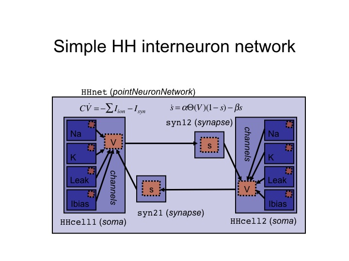
A graphical view of the chemical synaptic coupling in the Hodgkin-Huxley system demonstrated in the ModelSpec_test.py script (but omitting the gap junction) is: H-H model spec

3.3.2. Non-dynamic synapse with associated transition function

This is not currently implemented. An example would be the so-called "alpha function" post-synaptic timecourse function.

In order to implement this in the future, the connectWithSynapse function would be adapted to not create a synapse class instance, but to create a post-synaptic channel term in the target cell's compartment for which the gating variable is given by an explicit function of the pre-synaptic voltage, rather than a differential equation.

3.3.3. Adaptive synapses (facilitation and depression)

We support a maximum of two synaptic variables per synaptic connection, which can be coupled together in a way that provides a simple model of facilitation or depression. An example of implementing facilitation is given in the \tests\CIN.py example script, using the makeAdaptingSynapse function.

3.3.4. Threshold functions

Users can specify their own voltage-threshold functions, for use in trigering a post-synaptic response. The default function is 0.5+0.5*tanh(V/4), where the voltage threshold is set at 0 mV.

3.3.5. Removing synaptic connections

The disconnectSynapse function undoes the creation of the synaptic channel in the target cell, and removes all associated entries in the target cell's ModelSpec registry. The synapse object is not actually deleted, in case the user wishes to re-use it later.

3.4. Electrical (gap junction) synapses

3.5. Second messengers

We now support ionic current models that involve second messengers such as calcium. These are demonstrated in /tests/ModelSpec_test.py.

4. DSSRT toolbox

This is demonstrated in /tests/HH_DSSRTtest.py. This toolbox supercedes the export tools for the original Matlab version of DSSRT discussed in Section 4.1. DSSRT stands for Dominant Scale System Reduction Tool.

4.1. Tools for interfacing with DSSRT in Matlab

This toolbox provides utilities to export ODE models in PyDSTool to the analysis software package DSSRT, written in Matlab. The Matlab implementation works only for "conditionally linear" systems such as conductance-based neural networks, chemical kinetics netorks, and many other systems that can be written using a "kinetic" formalism.

The primary class of this toolbox is DSSRT_info. A single instance of it need not be initialized with any arguments, but there is an optional finite approximation to infinity, which defaults to 1e10. To trap bound violations this value can be dropped to a very modest finite number (e.g. in the '00s).

The makeDSSRTcfg method of this class is the intended access point for a user, but at this time is not fully implemented. To this method the user must supply a Model class instance containing a single ODE system Generator, and also the ModelSpec instance that defines it. The reason for this is that this method will only know how to convert a model to DSSRT format if it was created using the neuralcomp toolbox, described earlier on this page.

In lieu of the makeDSSRTcfg method, the class instance must be configured interactively. What follows is an example slightly adapted from a script for a stomatogastric ganglion model configuration, for which the object STG is an ODE Generator.

STG_dssrt = DSSRT_info('STG_PD', infty_val=120)

STG_dssrt.prepVarNames( ['PDa_Kd_m', 'PDa_L', 'PDa_Na_h', 'PDa_Na_m', 'PDa_V', 'PDs_A_h', 'PDs_A_m', 'PDs_Ca', 'PDs_CaS_m', 'PDs_CaT_h', 'PDs_CaT_m', 'PDs_I', 'PDs_KCa_m', 'PDs_Kd_m', 'PDs_L', 'PDs_NaP_h', 'PDs_NaP_m', 'PDs_V', 'PDs_h_m'])
dummyvars = ['PDs_L', 'PDs_I', 'PDa_L']
STG_dssrt.deqns = remain(remain(STG_dssrt.varsall, STG.funcspec.auxvars), dummyvars)
STG_dssrt.prepInputs(STG.funcspec.dependencies)
subsFnDef, not_depars = STG_dssrt.prepAuxFns(auxfndict, default_pars, makeMfiles=makeMfiles)
assert not_depars == []  # make sure all were DE pars
gate_m = ['PDs_CaT_m', 'PDs_CaS_m', 'PDs_h_m', 'PDs_NaP_m', 'PDs_Kd_m',
            'PDs_KCa_m', 'PDs_A_m', 'PDa_Na_m', 'PDa_Kd_m']
STG_dssrt.setUnitBounds(['PDs_L', 'PDs_I', 'PDa_L'] \
                         + gate_m + int_var_specs.keys())
for v in ['PDa_V', 'PDs_V']:
    STG_dssrt.bounds[v] = [-60, -20]
STG_dssrt.bounds['PDs_Ca'] = [0, 25]
STG_dssrt.cfac = {'PDs_V': 'PDs_Cm', 'PDa_V': 'PDa_Cm'}
STG_dssrt.depars = default_pars
STG_dssrt.prepDEpars()
STG_dssrt.prepGraph(vbars_int={'PDs_CaT_h': 'PDs_CaT_m',
                               'PDs_NaP_h': 'PDs_NaP_m',
                               'PDs_A_h': 'PDs_A_m',
                               'PDa_Na_h': 'PDa_Na_m'})
plotNetworkGraph(STG_dssrt)
# display information about the setup
info(STG_dssrt, "STG DSSRT setup")
STG_dssrt.outputCFG('STG_PD')

When the DSSRT_info object has been configured, the DSSRT files can be created in the file system using the method call outputCFG(<filename>), which includes the .cfg file. However, at this time, the specification of the GAMMA1TERMS and GAMMA2TERMS in the .cfg file still have to be filled in by hand before the files are ready for use in DSSRT. See the DSSRT documentation for details.

The DSSRT_info class makes use of the Fruchterman-Reingold graph drawing algorithm, provided in FR.py, in order to turn the connectivity network of an ODE system (where variables are nodes and their interconnections are links) into a convenient 2D graph representation.

5. Phase plane tools

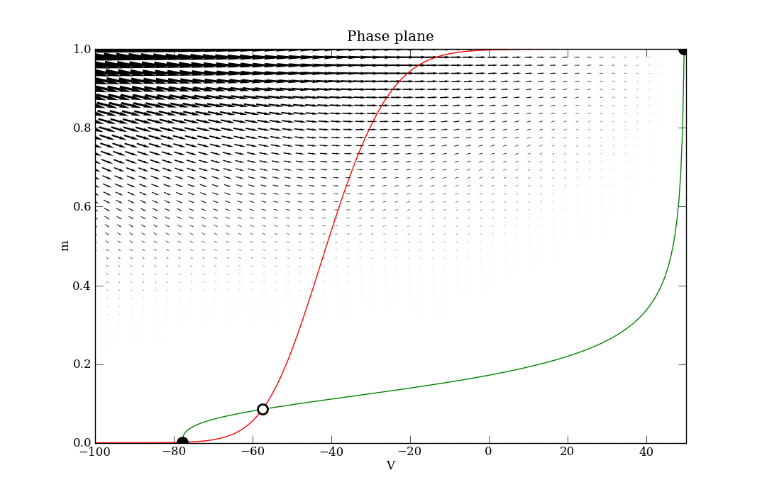
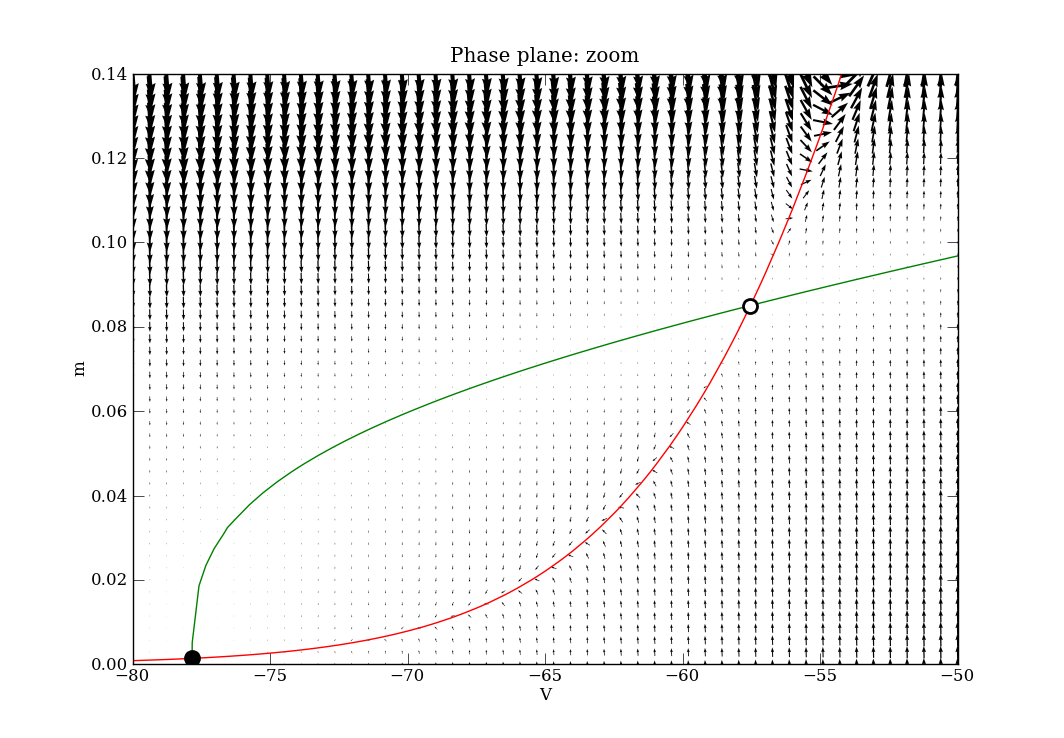
The code is well commented and the API documentation is detailed. A couple of appropriately named examples are also present in the tests directory. The first one to look at is Tutorial_VdP.py, which has its own tutorial page here. After that, see phaseplane_HHtest.py. In the latter, the following phase plane diagrams are produced for the (V, m) sub-space of the variables in the 4-D ODE system. The script shows a combination of calls for finding fixed points, nullclines and the vector field, and how to plot them effectively.

Classes defined

Functions defined

5. Phase response curves

The adjoint PRC calculation can be performed on an oscillator for which there exists a normally hyperbolic stable limit cycle. For direct PRC calculations the functions in InputProfile.py help to set up the database model of input signal to the oscillator. See the recent paper in Neural Computation by Govaerts and Sautois and the scholarpedia page on PRCs for details of both calculations.

6. Mechanical modeling

This toolbox contains matrix utilities for mechanical modeling, such as for augmenting position or displacement 3-vectors to 4-vectors, and constructors for spatial transformations.

An example of a rigid-body ODE/DAE system describing finger motion (using equations for an inverted triple pendulum with non-constant mass matrices) are found in PyDSTool/tests/freefinger_noforce_radau.py.

7. Fractal dimension analysis

Correlation and pointwise dimension analysis tools for time-series data analysis. For more information on pointwise dimension see J. Guckenheimer, "Dimension Estimates for Attractors", Contemporary Mathematics, Vol. 28, 1984. A journal publication concerning the use of these functions has been published in IEEE Transactions on Biomedical Engineering (see the an extended version at the arXiv). The prep_boxplot.py functions provide plotting tools for the results of our pointwise dimension estimation algorithm PD-E, described in detail in the journal paper.

8. Data analysis

Data analysis tools and utilities, particularly involving estimation of dimension in data-driven modelling, using principal component analysis (PCA). This toolbox requires the MDP Modular toolkit for Data Processing package.

Toolbox Documentation

1. Disclaimers