- Overview
- Types of curves, points and bifurcations supported
- A first look at PyCont
- Examples
- Classes and methods
- Plotting
- Details of algorithmic implementation
1. Overview
PyCont was originally written and maintained by Drew LaMar at Cornell University as part of John Guckenheimer's research group (Drew is now working at The College of William and Mary). PyCont is a sub-package of PyDSTool that provides tools for numerical continuation (a.k.a. path following) for solutions to initial value problems (IVPs, in the form of ODEs and discrete maps) and level curves of nonlinear functions. It also detects bifurcation points. For an introduction to bifurcations see this page on Scholarpedia.
The principal elements of performing continuation using PyCont are the specification of a system, determination of the type of continuation problem to study with that system, and finally the choice of methods to study that problem.
PyCont is currently implemented in pure Python (except the interface to AUTO), although it relies on user-specified "call-back" functions that are provided by Model or Generator objects. Thus, functions for vector fields and maps may be specified by C code as part of a Generator that is present as a dynamically-linked library. This can provide a substantial improvement to the efficiency of loops involving heavy use of these call-back functions.
2. Types of curves, points and bifurcations supported
The following curve types are handled by PyCont:
EP-C Equilibrium point curve
LP-C Limit point curve/Fold curve/Saddle-node curve
H-C1 Hopf point curve (method 1)
H-C2 Hopf point curve (method 2)
FP-C Fixed point curve (discrete systems)
LC-C Limit cycle curve (interface to AUTO)
as well as detection of the following bifurcations associated with one or more of the curves above:
LP Limit Point/Fold point/Saddle-node (EP-C)
H Hopf Point (EP-C)
BP Branch Point (EP-C)
CP Cusp Point (LP-C)
BT Bogdanov-Takens Point (LP-C, H-C1, H-C2)
ZH Zero-Hopf Point (LP-C, H-C1, H-C2)
GH Generalized-Hopf Point (H-C1, H-C2)
DH Double-Hopf Point (H-C1)
LPC Limit point of cycles (FP-C, LC-C)
PD Period doubling (FP-C, LC-C)
NS Neimark-Sacker/Torus bifurcation (FP-C, LC-C)
There are also the following point types for all curves (except RG) not associated with bifurcations:
P Endpoint
RG Regular point (LC-C)
MX Termination point
B Boundary point of computational domain
The point type RG is created based on the parameter NumSPOut. The point type MX is associated with some type of computational difficulty. It usually represents non-convergence based on our tolerances, but for many different reasons (e.g. initial point is too far from the requested curve type, too close to a homoclinic (large period), ...) The point type B indicates that a continuation parameter reached a boundary specified by pdomain to the dynamical system.
Support for continuation of periodic orbits is available via a low-level interface to the AUTO package. This requires an external C compiler to be accessible to Python via distutils, in the same way as is needed for the ODE integrators Radau and Dopri (see the GettingStarted page for set-up help).
2.1. Limitations
Bifurcations of ODEs with mass-matrix specifications and continuous-valued hybrid systems (not those that can be expressed as maps) are not yet supported.
Boundary value problems are not yet supported.
3. A first look at PyCont
3.1. Level sets of functions
PyCont can be used to find zero level sets of nonlinear functions. All that has to be done is to select a coordinate to use as a parameter, and specify the function as if it was the right hand side of an ODE. In other words, to find a solution (x(s), y(s)) parameterized by s of f(x,y) = C we treat x (say) as a parameter and study the one dimensional IVP y' = f(x, y) - C .
This representation enables the standard syntax for defining a differential equation in PyDSTool, but is only a way to provide PyCont with the function whose zero value in (x,y) space must be followed. The initial condition to the system can be any value of y that is close to a solution of the problem (PyCont will improve this point if it's not close enough before starting continuation). This should correspond to the initial value for the parameter x chosen.
Here is the example PyCont_LevelCurve.py:
   1 """Using PyCont to do path following to find a zero level set of a nonlinear
   2 function. Example is an ellipse.
   3
   4 Robert Clewley, August 2008.
   5 """
   6
   7 from PyDSTool import *
   8
   9 # f(y) = 0 is the required form
  10 # where f(y) = x^2 /2 + y^2 - 1
  11 DSargs = args(name='ellipse')
  12
  13 # treat one of the coordinates as a parameter for PyCont to use
  14 DSargs.pars = {'x': 0}
  15
  16 # the other coordinate is a 'variable'
  17 DSargs.varspecs = {'y': 'x*x/2.+y*y-1'}
  18
  19 # A starting point on the ellipse, if known. Let's pretend it's a tougher
  20 # problem and we only know a point that's close to it: (x,y) = (0, 1.1)
  21 # PyCont will find the closest point that's actually on the curve before
  22 # doing the path following
  23 DSargs.ics = {'y': 1.1}
  24
  25 # Define an initial value problem (ODE) with f(x) as the right hand side.
  26 # For this example, it is just a formality to present PyCont with f(x).
  27 # In examples involving fixed points or limit cycles of dynamical systems,
  28 # this ODE will have a practical meaning.
  29 testODE = Vode_ODEsystem(DSargs)
  30
  31 # Create an instance of PyCont
  32 P = ContClass(testODE)
  33
  34 # EP-C = equilibrium point curve
  35 PCargs = args(name='test', type='EP-C')
  36 PCargs.freepars = ['x']
  37 PCargs.StepSize = 1e-3
  38 PCargs.MaxNumPoints = 800
  39 PCargs.MaxStepSize = 1e-2
  40
  41 # Declare a new curve based on the above criteria
  42 P.newCurve(PCargs)
  43
  44 # Do path following in the 'forward' direction. Max points is large enough
  45 # to ensure we go right around the ellipse (PyCont automatically stops when
  46 # we return to the initial point - unless MaxNumPoints is reached first.)
  47 P['test'].forward()
  48
  49 sol = P['test'].sol
  50
  51 print "There were %i points computed" % len(sol)
  52 # solution points:
  53 print sol
  54
  55 print "\nLabels for each point in sol pointset give diagnostic information about"
  56 print "first derivative of the point along the curve ('V' entry) and the arc "
  57 print "length parameter shows distance along the curve so far ('ds' entry)."
  58
  59 print "\nVelocity around curve is always 1, e.g. look at 100th point"
  60 print "norm(Point(sol[100].labels['EP']['data'].V)) =", \
      norm(Point(sol[100].labels['EP']['data'].V))
  61
  62 print "... at which we have travelled distance ds =", \
      sol[100].labels['EP']['data'].ds
  63
  64 print "\nThis distance is equal to 100 * the max step size (0.01) which PyCont"
  65 print "deemed sufficient for the desired accuracy."
  66
  67 # easy way to plot the result
  68 P.display(curves=['test'], coords=('x','y'))
3.2. For initial value problems
In the simplest terms, an instance of the PyCont continuation class is created for a given model object that defines an ODE or a map system, and a selection of algorithmic parameters. These parameters determine the type of continuation desired for the system, and the free parameter(s) to be used. The PyCont instance contains any number of curves associated with the same system.
The PyCont instance may then continue from an initial state (a point or a cycle) for a particular solution curve, using the forward or backward class methods. Computation ends when continuation fails or the maximum number of steps is reached. Repeated calls to these methods will extend the computed solution curve.
If a PyCont instance named pc contains a curve named 'EQ' then the labelled solution curve is saved as a Pointset object, in the attribute pc['EQ'].sol.
Solution curves can be plotted using calls such as pc['EQ'].display() for specific curves, or pc.display() for all curves on the same diagram.
3.3. Screenshots
3.3.1. A-->B Reaction
3.3.2. Lorenz System
4. Examples
There are many examples provided in the PyDSTool/tests/ directory. Each one starts with "PyCont_". The docstring and comments in each file provide more information. Currently, there are demo scripts for:
a simple saddle node bifurcation demo
computing level sets of functions
chemical reaction kinetic equations (ABC, AB, Brusselator, Catalytic)
discrete and continuous predator prey models
the Lorenz system
a Hamiltonian system
the Logistic model
the Hopfield model (courtesy of David Sterratt)
the van der Pol relaxation oscillator
Various biophysical neuron models (Hindmarsh Rose, Morris Lecar, and a Lateral Pyloric neuron)
4.1. Worked example: Catalytic Oscillator
It's easiest to illustrate the usage of PyCont by working through one of the examples in the PyDSTool/tests directory. Let's look closely at the example PyCont_Catalytic_demo.py. The following block of code initializes the model using PyDSTool conventions. The last line creates an instance of the class ContClass tied to the model just created using PyDSTool:
   1 from PyDSTool import *
   2
   3 pars = {'q1': 2.5, 'q2': 1.92373, 'q3': 10, 'q4': 0.0675, 'q5': 1, 'q6': 0.1, 'k': 0.4}
   4
   5 icdict = {'x': 0.0014673, 'y': 0.826167, 's': 0.123119}
   6
   7 auxfndict = {'z': (['x', 'y', 's'], '1 - x - y - s')}
   8
   9 xstr = '2*q1*z(x,y,s)*z(x,y,s) - 2*q5*x*x - q3*x*y'
  10 ystr = 'q2*z(x,y,s) - q6*y - q3*x*y'
  11 sstr = 'q4*z(x,y,s) - k*q4*s'
  12
  13 DSargs = args(name='CatalyticOscillator')
  14 DSargs.pars = pars
  15 DSargs.varspecs = {'x': xstr, 'y': ystr, 's': sstr}
  16 DSargs.fnspecs = auxfndict
  17 DSargs.ics = icdict
  18
  19 testDS = Generator.Dopri_ODEsystem(DSargs)
  20 PyCont = ContClass(testDS)
We are now ready to create continuation curves for this model. The next block of code creates a "struct"-like data type of parameters (that can also be treated like a dictionary), which specifies an equilibrium curve:
   1 PCargs = args(name='EQ1', type='EP-C')   # as many arguments can be supplied here as desired
   2 PCargs.freepars = ['q2']   # rest of the arguments created like a struct
   3 PCargs.StepSize = 1e-3
   4 PCargs.MaxNumPoints = 175
   5 PCargs.MaxStepSize = 1e-2
   6 PCargs.LocBifPoints = ['LP','H']
   7
   8 PyCont.newCurve(PCargs)
   9 PyCont['EQ1'].forward()
The type parameter is labeled EP-C, which stands for an Equilibrium Point Curve. Note that there is only one free parameter for this type of curve. LocBifPoints specifies which types of bifurcation points to detect. In this case, we are detecting limit points (LP) and hopf points (H). We then call the newCurve() method of the PyCont instance, passing the parameter dictionary as an argument. Once it is created, we refer to it by name and call its forward() method to compute the curve. There will be output stating that two limit points and two hopf points were detected. At this point, once computation has finished, we can view the results two ways, given by the following code:
1 PyCont['EQ1'].info()
The first method info() will spit out various information about the curve, such as continuation parameters and special points that were detected. Under the special points, you will see P1, P2, LP1, LP2, H1, H2 denoting the two limit points and two hopf points that were detected. P1 is a label for the starting point and P2 a label for the ending point. You can access these points from the curve by the following:
   1 X = PyCont['EQ1'].getSpecialPoint('LP1')
   2 print X
If the point exists (which it does in this case), it will return that point on the curve as a Point class object. Any bifurcation information that was found for that point can be found in the data structure X.labels['LP']['data'], where X was the returned special point. For example, the following gives the normal form information for the limit point LP1:
1 X.labels['LP']['data'].a
Now we want to plot the results:
   1 PyCont['EQ1'].display(axes=(1,2,1))
   2 PyCont['EQ1'].display(('q2','x'), axes=(1,2,2))
   3 PyCont.plot.info()
If you don't send display() arguments, it will default to the coordinates consisting of the first free parameter and the first listed state variable. The second line lets you specify the plotting coordinates. You will notice that the special points are labeled and colored according to their type. Notice also that we are specifying the axes using subplot notation from Matlab. PyCont has a plotting structure, PyCont.plot, that stores all of the matplotlib handles to the objects in the plots. You can query its info() method to see the organizational hierarchy. We will give examples of the functionality of the plotting class later in the demo. Also, if you happen to forget what the parameters or variables are for the model when you want to plot, you can quickly access them by typing:
1 PyCont.info()
Now that we have an equilibrium curve, let's continue a hopf curve starting from one of the special points computed above. The following block of code sets up and computes a hopf curve from the special point H2:
   1 PCargs = args(name='HO1', type='H-C2')
   2 PCargs.initpoint = 'EQ1:H2'
   3 PCargs.freepars = ['q2', 'k']
   4 PCargs.MaxStepSize = 1e-2
   5 PCargs.LocBifPoints = ['GH', 'BT', 'ZH']
   6 PCargs.MaxNumPoints = 100
   7
   8 PyCont.newCurve(PCargs)
   9 PyCont['HO1'].forward()
The type now is H-C2, standing for Hopf curve using method 2. The initial point is specified by label as EQ1:H2, meaning special point H2 on curve EQ1. In general, you can specify an initial point as a dictionary, a Point, a label, or an array. For a curve of this type, we need two free parameters, so we free up the extra parameter k. LocBifPoints is now set to detect GH, BT and ZH points.
Note: You may have noticed that we didn't specify an initial point for EQ1 above. When an initial point is not specified, it defaults to the initial conditions for the model. Also, the initial point is checked to see if it is of the right type and, if it is not, it is corrected to the "closest" point of that type.
The output of forward() is the location of two GH points. You can type PyCont['HO1'].info() to get information on the curve, or you can type PyCont['HO1'].display() to plot the results. What I want to point out now, however, is what happens when you do the following:
   1 PyCont.plot.clearall()
   2 PyCont.display(('q2','x'))
The first line clears all open figures (in this case just fig1). The second line plots all computed curves for the PyCont class, in this case EQ1 and HO1, to the just-cleared active figure fig1.
Let's now compute a curve of fold points starting from LP1:
   1 PCargs = args(name='FO1', type='LP-C')
   2 PCargs.initpoint = 'EQ1:LP1'
   3 PCargs.freepars = ['q2', 'k']
   4 PCargs.LocBifPoints = 'all'
   5 PCargs.MaxNumPoints = 110
   6
   7 PyCont.newCurve(PCargs)
   8 PyCont['FO1'].forward()
This is a limit point curve, denoted LP-C, starting from the point EQ1:LP1. We use the same free parameters as for the hopf curve. For LocBifPoints, we now specify that we want to compute all bifurcation points for this curve type, which in the fold case are BT, CP, and ZH points.
We plot all curves as before:
   1 PyCont.plot.clearall()
   2 PyCont.display(('q2','x'))
We could have just as easily typed PyCont['FO1'].display(('q2','x')), and the curve FO1 will have been added to the existing figure. Let's now move backward along the fold curve:
1 PyCont['FO1'].backward()
Since we've added more points to the fold curve, we want to update the plot to show the changes. The plotting program is not extremely intelligent here to know which points on the curve have already been plotted, so we must delete the existing FO1 curve from the plotting class and replot the FO1 curve. The following commands perform these actions:
   1 PyCont.plot.fig1.axes1.FO1.delete()
   2 PyCont['FO1'].display(('q2','x'))
Let's now look more closely at what else the plotting class can do. The plots can get pretty cluttered with points and labels, so we've included an option to toggle labels, points, curves and cycles on and off. The following command toggles the labels in all figures and axes off:
1 PyCont.plot.toggleLabels('off')
Now consider the actions of the following commands:
   1 PyCont.plot.toggleLabels('on')
   2 PyCont.plot.togglePoints('off')
   3 PyCont.plot.toggleCurves('off', byname='HO1')
   4 PyCont.plot.fig1.axes1.HO1.toggleCurve('off')
The first line toggles all labels back on in all plots. The second line toggles all points off, while the third line toggles an entire curve (labels and points included) off by specifying it's name, in this case curve HO1. You can perform the same operation by traversing through the plot class to the curve and using the singular method, toggleCurve(). The fourth line does just that, although it's redundant in its actions.
Eigenvalues are by default not computed along the curve. You can compute them afterwards, however, and represent the stability of the equilibrium points in a new plot as follows:
   1 PyCont.computeEigen()
   2 PyCont.display(coords=('q2','x'), stability=True, figure='fig2')
   3 PyCont.plot.fig2.toggleAll('off', bytype='P')
Stable fixed points are represented as solid lines, unstable fixed points as dashed lines, and neutral fixed points as dashed/dotted lines. There is some ambiguity in the situation where there is a stream of fixed points which change stability at each step. In this situation, the curve is drawn as a dotted line. Reducing MaxStepSize and computing again may resolve this ambiguity. Also, in computing limit cycle curves, sometimes the Floquet multipliers are inaccurate. In this case, the curve will also be drawn as a dotted line. This is pretty common in the case where a limit cycle vanishes in a homoclinic orbit. See PyCont_Lorenz.py and zoom in on the endpoints. The third and final line uses a method called toggleAll for figure fig2. It turns special points on or off (both labels and points). Here we specify all points that are endpoints (type P). The endpoints are useful to know what is forward or backward in computations (P1-->P2 is forward), but once you want to publish the picture, they are unnecessary, so we turn them off. This is a common procedure in a lot of the examples. All of the plot methods can be applied at any level in the hierarchy, so you can, for example, toggle all labels off in a specific figure, axes, curve or point.
One thing that is not mentioned in this example is the ability to perform matplotlib commands on any object that PyCont has created. You can access the matplotlib handles to the objects (such as figures, axes, curves, points, and texts) within the plot class. For example, if you ran the demo in interactive mode (using python -i), you can now type:
   1 PyCont.plot.fig2.axes1.axes.set(xlabel='Free Parameter: q2')
   2 PyCont.plot.refresh()
This will access the axes handle and allow you to perform whatever command you want directly. The second line recursively goes through the plot class and performs a pylab.draw() on all figures and axes so that you can see the change. See Plotting below to see how to access the other objects.
4.2. Respecting user-defined bounds on the parameters
In the Hopfield model example PyCont_Hopfield.py PyCont will stop at the pre-determined bounds of the parameters given by the pdomain to DSargs if continuation reaches either end of that domain. That is specified by setting PCargs.StopAtPoints = ['B'].
4.3. Note about user-defined functions for continuation
User-defined continuation functions are introduced in PyCont_vanDerPol.py, where canards are computed. This involves a sophisticated (read: not altogether user-friendly) way of adding an event to the system that is then manipulated within a user-specified function cont_func in the body of the file, which is then passed as the continuation function to PyCont. This functionality is used to track canards in the van der Pol system.
5. Classes and methods
5.1. ContClass
This is the main class which represents one continuation session. This class will hold all curves computed for a particular generator/model created by PyDSTool. Once curves exist, you can display them all at once using its display() method and toggle the plotted labels on and off with the toggleLabels() method. The following will initialize a continuation session:
session = ContClass(model)
where model is a Model or Generator instance.
5.1.1. Attributes/Parameters
5.1.2. Methods
5.1.2.1. newCurve()
Syntax
newCurve(args)
Description
Creates a new curve. args is a dictionary of parameters for the curve. Required parameters upon initialization are:
type: String specifyng curve type (EP-C, LP-C, H-C1, H-C2)
name: String specifying the curves name
initpoint: Initial point (of type Point, dict, array, list, or label). If this is not specified, it will default to the initial condition for the model. If this does not exist, an error will result. If a label is given, it should be given as a string in the format <curve name>:<point label>. For example, if the label of a limit point is LP1 from a curve named EQ1, then initpoint should be EQ1:LP1.
initdirec: Initial direction along curve (of type dict). If this is not specified, it will be computed. This is used, for example, when continuing along a second branch of a curve. To see its usage, see the example PyCont_Logistic.py.
freepars: List of strings specifying the free parameters. If this is not specified, it will default to the first number of parameters listed in the model that are necessary for the continuation of a curve of the type specified in type.
Defaults will be given for the remaining parameters. For a list of parameters, see ???.
5.1.2.2. update()
Syntax
update(args)
Description
Update parameters for all curves. args is a dictionary of parameters from the list below:
verbosity (0 = no output, 1 = minimal output, 2 = full output)
5.1.2.3. display()
Syntax
display(coords=None, curves=None, figure=None, axes=None, stability=False, **plot_args)
Description
Displays computed curves listed in curves, otherwise display all curves.
coords: (None/tuple) If this is None, the x-coordinate will be the first listed free parameter and the y-coordinate the first listed state variable. If this is a tuple, the coordinates can be chosen from the state variables and parameters, including auxiliary parameters, such as period _T (see LC-C) or _k (see H-C2).
curves: (None/list of strings) If this is None, then all curves will be displayed. Otherwise, it should be a list of curve names.
figure: (None/string) If this is None, then either the current figure will be the active figure or a new figure will be opened and become active. As a string, this represents the name of the figure to display the curves. If the figure name does not currently exist, a new figure is opened.
axes: (None/string/tuple) If this is None, then either the current axes will be the active axes or a new axes will be opened and become active. As a string, this represents the name of the axes to display the curves. If the axes name does not currently exist, a new axes is opened. As a tuple (n,m,i), this represents the i-th m x n subplot of the active figure.
stability: If eigen information is stored, then when this flag is True, stability information is plotted. Stable (S) fixed points are drawn as solid lines, unstable (U) as dashed lines, and neutral (N) as dashed-dotted lines. There is a fourth category (X), drawn as dotted lines, for the ambiguous situation where there is a stream of fixed points that changes stability at each step. Reducing MaxStepSize may resolve this ambiguity.
plot_args: Any argument that you would pass to the pylab.plot() command, such as linewidth or label, can be given here to be applied to all curves displayed.
Note: If you are using a backend other than TkAgg, you will not have interactive plotting (see matplotlib). Also, in order to see the plot after the display() command, you need to run the extra command show().
5.1.2.4. info()
Syntax
info()
Description
Displays information on the curve. The information includes:
model
state variables
model parameters
curves (names and types)
5.1.2.5. computeEigen()
Syntax
computeEigen()
Description
Computes the eigen information along all curves. The resulting eigenvalues, eigenvectors (right) and stability are stored as data along the curve in the attribute sol. For example, if you are continuing an equilibrium curve (EP-C), it will be located as follows:
sol[n].labels['EP']['data'].evals
sol[n].labels['EP']['data'].evecs
sol[n].labels['EP']['stab']
The stability is denoted as S for stable, U for unstable and N for neutral. Once the eigen information is computed and stored, the stability information can be plotted with the curve. See display() for details.
5.1.2.6. exportGeomview()
Syntax
exportGeomview(coords=None, filename="geom.dat")
Description
Useful for 3-dimensional plots. This method is called by display() when coords is 3-dimensional. It will export all curves to the file filename for importing into the geometric viewing program Geomview.
coords=None: See display(). This must be length 3.
filename="geom.dat": File where Geomview output is stored.
5.2. Curve classes (EP-C, LP-C, H-C1, H-C2, FP-C, LC-C)
Once a curve is created by the newCurve() method of ContClass, you can access it by name using the following syntax:
ContClass[<curve name>]
For example, if the curve name is EQ1, then ContClass['EQ1'] represents the curve. The following lists the attributes and methods for the curve classes.
5.2.1. Attributes/Parameters
Always use the update() method to change or set parameters.
5.2.1.1. MaxNumPoints
Type
Float
Description
Maximum number of points to compute along the curve for a specific call of forward or backward.
5.2.1.2. MaxCorrIters
5.2.1.3. MaxTestIters
5.2.1.4. MaxStepSize
Type
Float
Description
Maximum step size.
5.2.1.5. MinStepSize
Type
Float
Description
Minimum step size.
5.2.1.6. StepSize
Type
Float
Description
Initial step size. The step size will be adapted along the curve based on convergence criterion and will not exceed the bounds specified by MinStepSize and MaxStepSize.
5.2.1.7. VarTol
Type
Float
5.2.1.8. FuncTol
Type
Float
5.2.1.9. TestTol
Type
Float
5.2.1.10. ClosedCurve
Type
Bool
5.2.1.11. LocBifPoints
Type
List
Description
Don't set this if you don't want to detect any bifurcations. Set it to 'all' to detect all types, or give a list of string symbols for any of the types listed in Section 7 below, i.e. any of LP, H, BP, CP, BT, ZH, GH, DH, LPC, PD, NS, and the parameter boundary B (if defined by pdomain in your dynamical system).
5.2.1.12. StopAtPoints
Type
List
Description
Sets the bifurcations that, when detected, will stop the continuation algorithm. Uses the same codes as LocBifPoints (see above).
5.2.1.13. SaveJacobian
Type
Bool
Description
Calculates and saves the jacobian along the curve. The jacobians are stored in the sol pointset for each point on the curve in their respective data field. For all curve types except LC-C, the jacobians with respect to the state variables and parameters are saved respectively as jacx and jacp. For example, if you just computed an equilibrium curve and named it 'EQ1', you could find it as PyCont['EQ1'].sol[#].labels['EP']['data'].jacx. For curve type LC-C, the jacobian represents the jacobian of the flow. It is saved in two pieces as jac0 and jac1. If you explicitly want the jacobian of the flow, it is given by inv(jac1)*jac0, where inv represents the inverse of a matrix.
5.2.1.14. SaveEigen
Type
Bool
Description
Calculates and saves the eigenvalues along the curve. The eigenvalues are stored in the sol pointset for each point on the curve in their respective data field. The eigenvalues are saved as evals.
5.2.1.15. verbosity
Type
Integer
Description
Controls amount of output to the screen. 0 is none, 1 minimal, and 2 full output.
5.2.1.16. period [FP-C]
Type
Integer
Description
Specifies the period of the cycles you want to continue. This is especially important if you want to compute the period doubling branch at a PD point. This will be somewhat automated in the future. See PyCont_Logistic.py.
5.2.1.17. SolutionMeasures [LC-C]
Type
String/List of strings
Description
Specifies which solution measures to compute along the limit cycle curve. The solution measures are:
max: Maximum of each cycle component.
min: Minimum of each cycle component.
avg: Average of each cycle component.
nm2: L2 norm of each cycle component.
Default is to compute max along the curve. We'll use an example to illustrate accessing these measure in the computed solution. Suppose we have the coordinate u1 in our system and we've asked for avg. Then there will be a coordinate named u1_avg in the computed pointset sol.
5.2.1.18. NumSPOut [LC-C]
5.2.1.19. NumIntervals [LC-C]
5.2.1.20. NumCollocation [LC-C]
5.2.1.21. AdaptMesh [LC-C]
5.2.1.22. DiagVerbosity [LC-C]
5.2.2. Methods
5.2.2.1. update()
Syntax
update(args)
Description
Update the continuation parameters. args is a dictionary of parameters for the curve.
5.2.2.2. reset()
Syntax
reset(args)
Description
Reinitialize the curve to the parameters given in args. Anything not specified in args will be reset to its default value.
5.2.2.3. display()
Syntax
display(coords=None, figure=None, axes=None, stability=False, **plot_args)
Description
Display computed curve.
coords: (None/tuple) If this is None, the x-coordinate will be the first listed free parameter and the y-coordinate the first listed state variable. If this is a tuple, the coordinates can be chosen from the state variables and parameters, including auxiliary parameters, such as period _T (see LC-C) or _k (see H-C2).
figure: (None/string) If this is None, then either the current figure will be the active figure or a new figure will be opened and become active. As a string, this represents the name of the figure to display the curves. If the figure name does not currently exist, a new figure is opened.
axes: (None/string/tuple) If this is None, then either the current axes will be the active axes or a new axes will be opened and become active. As a string, this represents the name of the axes to display the curves. If the axes name does not currently exist, a new axes is opened. As a tuple (n,m,i), this represents the i-th m x n subplot of the active figure.
stability: If eigen information is stored, then when this flag is True, stability information is plotted. Stable (S) fixed points are drawn as solid lines, unstable (U) as dashed lines, and neutral (N) as dashed-dotted lines. There is a fourth category (X), drawn as dotted lines, for the ambiguous situation where there is a stream of fixed points that changes stability at each step. Reducing MaxStepSize may resolve this ambiguity.
plot_args: Any argument that you would pass to the pylab.plot() command, such as linewidth or label, can be given here to be applied to the curve.
Note: If you are using a backend other than TkAgg, you will not have interactive plotting (see matplotlib). Also, in order to see the plot after the display() command, you need to run the extra command show().
5.2.2.4. plot_cycles() [LC-C]
Syntax
plot_cycles(coords=None, cycles=None, figure=None, axes=None, normalized=False, color='default', **plot_args)
Description
Plots the cycles specified in cycles. For a description of figure and axes, see display() above.
coords: (None/tuple) If this is None, the x-coordinate defaults to time and the y-coordinate to the first state variable. If this is a tuple, the coordinates can be chosen from the state variables and parameters.
cycles: (None/string/list of strings) If this is not specified, all cycles will be displayed. A string or list of strings gives the name for the cycles (based on its associated special point on the limit cycle curve) to be displayed.
normalized: (True/False) If this is True, the period for each cycle will be scaled to 1 before plotting. This is only useful when you are plotting time on one of the axes.
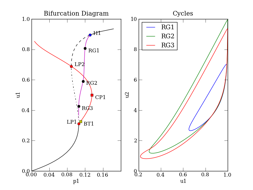
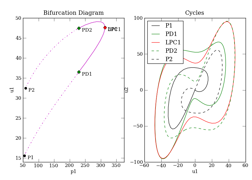
color: ('default', 'bytype') The default coloring will color the cycles in order through the default colormap. If 'bytype' is selected, the cycle color will be the color of its associated special point type on the curve. For example, period doubling points are colored green on the curve, so the period doubling cycles are also colored green (see PyCont_Lorenz.py).
plot_args: Any argument that you would pass to the pylab.plot() command, such as linewidth or label, can be given here to be applied to all specified cycles.
5.2.2.5. cleanLabels()
Syntax
cleanLabels()
Description
Reorders labels of all special points in the forward direction along the curve (i.e. from P1 to P2). For example, if you go forward along the curve and find a hopf point, it will be labeled H1. So the special point ordering will be P1 -> H1 -> P2. If you then go backward and find another hopf point, it will be labeled H2. Now the special point ordering will be P1 -> H2 -> H1 -> P2. Calling cleanLabels() will rename the special points to P1 -> H1 -> H2 -> P2.
5.2.2.6. forward()
Syntax
forward()
Description
Computes "forward" along the curve. The forward direction is chosen based on ...
5.2.2.7. backward()
Syntax
backward()
Description
Computes "backward" along the curve. See forward() above for a distinction between forward vs. backward.
5.2.2.8. getSpecialPoint()
Syntax
X = getSpecialPoint(label1, label2=None)
Description
Gets a special point on the curve specified by label1 and label2. The point, if it exists, is returned as a Point type.
X = getSpecialPoint(label1, label2): label1 specifies the point type. label2 specifies the point label.
X = getSpecialPoint(label1): label1 must be a point label of the form <point type #>, for example, LP3.
5.2.2.9. info()
Syntax
info()
Description
Displays information on the curve. The information includes:
curve name and type
model
continuation parameters
special points
5.2.2.10. computeEigen()
Syntax
computeEigen()
Description
Computes the eigen information along curve. The resulting eigenvalues, eigenvectors (right) and stability are stored as data along the curve in the attribute sol. For example, if you are continuing an equilibrium curve (EP-C), it will be located as follows:
sol[n].labels['EP']['data'].evals
sol[n].labels['EP']['data'].evecs
sol[n].labels['EP']['stab']
The stability is denoted as S for stable, U for unstable and N for neutral. Once the eigen information is computed and stored, the stability information can be plotted with the curve. See display() for details.
5.2.2.11. exportGeomview()
6. Plotting
PyCont contains a plotting class that helps keep track of your visual displays. The structure stores the handles to matplotlib figures, axes, curves, and points in a hierarchical fashion and is designed to make access to these handles easier than the built-in matplotlib interface. Some common and useful plotting tools, such as turning labels of points on or off or changing labels, is implemented through PyCont's plotting structure. This section covers the layout and structure of the plotting pargs class, as well as the methods implemented to handle useful plotting tools. The end of this section discusses how PyCont's plotting structure deals with other programs that manipulate matplotlib figures.
Note: If you are using a backend other than TkAgg, you will not have interactive plotting (see matplotlib).
6.1. pargs class
The pargs class is a recursively defined class that represents the hierarchy of plotting data. The root pargs class of the plotting data is an attribute plot in ContClass, as well as in each of the curve classes. Its structure is:
plot ---> figures ---> axes ---> curves/cycles ---> points
The pargs class is derived from the ancestor class args, and can thus be treated both as a structure and a dictionary. The pargs class attributes and methods are described below.
6.1.1. Attributes
6.1.1.1. plot
This contains pargs classes representing figures. Each figure is named starting from fig1.
6.1.1.2. figures
This contains the figure handle fig for this figure, as well as pargs classes representing axes. Each axes is named starting from axes1.
6.1.1.3. axes
This contains the axes handle axes for this axes, as well as pargs classes representing curves and/or cycles. Each curve is named according to its name given in PyCont, while each cycle is named according to its corresponding point name along the limit cycle curve.
6.1.1.4. curve
This contains the line2D handle(s) in the list curve. The length of this list is larger than one in the case where you plot stability, since the curve is broken into multiple pieces. This also contains pargs classes representing points along the curve.
6.1.1.5. cycle
This contains the line2D handle in the list cycle. There are no other attributes.
6.1.1.6. point
This contains two handles. The first is the line2D handle for the point itself in the list point. The second is the text label for the point in the handle text. There are no other attributes.
6.1.2. Methods
The recursive nature of the pargs class was designed so that all methods described below could be called at any level in the hierarchical plotting structure. For example, you can toggle the labels on or off for all points in a specific figure, axes, or curve.
6.1.2.1. info()
Syntax
info()
Description
Displays the hierarchical structure of the plots. It also displays the labels and legends for all curves, cycles and points, as well as curve types.
6.1.2.2. toggleLabels()
Syntax
toggleLabels(visible='on', bylabel=None, byname=None, bytype=None)
Description
Toggles the point labels on/off according to bylabel, byname, or bytype.
visible: Any string other than 'on' is considered 'off'.
bylabel: (string/list of strings) Turns on/off the point labels specified by the point labels listed here.
byname: (string/list of strings) Turns on/off the point labels specified by their respective point name in PyCont (e.g. H1, LP2, ...)
bytype: (string/list of strings) Turns on/off the point labels specified by their point type (e.g. H, LP, P, ...)
If bylabel, byname and bytype are all None, then all point labels will be turned on/off.
Note: When this is a method of a pargs class that represents a point, you can use the singular expression "toggleLabel(visible='on')" to toggle that specific point label on/off.
6.1.2.3. togglePoints()
Syntax
togglePoints(visible='on', bylabel=None, byname=None, bytype=None)
Description
Toggles the points on/off according to bylabel, byname, or bytype.
visible: Any string other than 'on' is considered 'off'.
bylabel: (string/list of strings) Turns on/off the points specified by the point labels listed here.
byname: (string/list of strings) Turns on/off the points specified by their name in PyCont (e.g. H1, LP2, ...)
bytype: (string/list of strings) Turns on/off the points specified by their point type (e.g. H, LP, P, ...)
If bylabel, byname and bytype are all None, then all points will be turned on/off.
Note: When this is a method of a pargs class that represents a point, you can use the singular expression "togglePoint(visible='on')" to toggle that specific point on/off.
6.1.2.4. toggleCurves()
Syntax
toggleCurves(visible='on', bylegend=None, byname=None, bytype=None)
Description
Toggles the curves on/off according to bylegend, byname, or bytype.
visible: Any string other than 'on' is considered 'off'.
bylegend: (string/list of strings) Turns on/off the curves specified by the curve legend labels listed here.
byname: (string/list of strings) Turns on/off the curves specified by their name in PyCont (e.g. EQ1, FO1, ...)
bytype: (string/list of strings) Turns on/off the curves specified by their curve type (e.g. EP, LP, H, ...)
If bylegend, byname and bytype are all None, then all curves will be turned on/off.
Note: When this is a method of a pargs class that represents a curve, you can use the singular expression "toggleCurve(visible='on')" to toggle that specific curve on/off.
6.1.2.5. toggleCycles()
Syntax
toggleCycles(visible='on', bylegend=None, byname=None, bytype=None)
Description
Toggles the cycles on/off according to bylegend, byname, or bytype.
visible: Any string other than 'on' is considered 'off'.
bylegend: (string/list of strings) Turns on/off the cycles specified by the cycle legend labels listed here.
byname: (string/list of strings) Turns on/off the cycles specified by their corresponding point name in PyCont (e.g. P1, PD1, ...)
bytype: (string/list of strings) Turns on/off the cycles specified by their corresponding point type (e.g. P, PD, LPC, ...)
If bylegend, byname and bytype are all None, then all cycles will be turned on/off.
Note: When this is a method of a pargs class that represents a cycle, you can use the singular expression "toggleCycle(visible='on')" to toggle that specific cycle on/off.
6.1.2.6. toggleAll()
Syntax
toggleAll(visible='on', bylabel=None, byname=None, bytype=None)
Description
Toggles the points, labels and cycles on/off according to bylabel, byname, or bytype.
visible: Any string other than 'on' is considered 'off'.
bylabel: (string/list of strings) Turns on/off all objects associated with the point labels listed here.
byname: (string/list of strings) Turns on/off all objects associated with their name in PyCont (e.g. H1, LP2, ...)
bytype: (string/list of strings) Turns on/off all objects associated with their point type (e.g. H, LP, P, ...)
If bylabel, byname and bytype are all None, then all objects (points, labels and cycles) will be turned on/off.
6.1.2.7. setLabels()
Syntax
setLabels(label, bylabel=None, byname=None, bytype=None)
Description
Sets all labels specified by bylabel, byname, or bytype to label.
label: (string)
bylabel: (string/list of strings) Sets the labels specified by the point labels listed here.
byname: (string/list of strings) Sets the labels specified by their name in PyCont (e.g. H1, LP2, ...)
bytype: (string/list of strings) Sets the labels specified by their point type (e.g. H, LP, P, ...)
If bylabel, byname and bytype are all None, then all point labels will be set to label.
Note: When this is a method of a pargs class that represents a point, you can use the singular expression "setLabel(label)".
6.1.2.8. setLegends()
Syntax
setLegends(legend, bylegend=None, byname=None, bytype=None)
Description
Sets legends of all curves or cycles specified by bylegend, byname, or bytype to legend.
legend: (string)
bylegend: (string/list of strings) Sets the legends specified by the curve or cycle legends listed here.
byname: (string/list of strings) Sets the legends specified by their name in PyCont (e.g. EQ1 for a curve, LPC1 for a cycle, ...)
bytype: (string/list of strings) Sets the legends specified by their curve type (e.g. H, LP, P, ...) OR cycle type (e.g. LPC, PD, ...)
If bylegend, byname and bytype are all None, then all curve/cycle legends will be set to legend.
Note:  When this is a method of a pargs class that represents a curve or a cycle, you can use the singular expression "setLegend(label)".
Note 2: This needs to be called separately for cycles and curves.
6.1.2.9. clear()
Syntax
clear()
Description
Clears the corresponding object as follows:
figure: Removes all axes in the figure.
axes: Removes all objects in the axes.
curve: Removes all points on the curve.
point: This is the same as delete.
6.1.2.10. clearall()
Syntax
clearall()
Description
Calls clear() on all objects in that level of the plotting hierarchy.
6.1.2.11. delete()
Syntax
delete()
Description
This calls clear() on the current object and then deletes it.
6.1.2.12. deleteall()
Syntax
deleteall()
Description
Calls delete() on all objects in that level of the plotting hierarchy.
6.1.2.13. refresh()
Syntax
refresh()
Description
Refreshes that object in the display.
Note: Calling at the level of `plot` will refresh all figures.
6.1.2.14. clean()
Syntax
clean()
Description
Goes through the plotting structure and performs maintenance. If any outside program (whether it be software or human) modified the displays in any way, such as closing figures by hand or through pylab, this method needs to be called so that it can delete old handles. This is called automatically before every display() command, so if you've closed a figure by hand, it will correct itself most of the time on its own. When you do close a figure by hand, the current method to detect that it has been closed is to spawn a dummy figure and then close it immediately, so don't be surprised if you see a figure flicker on and off.
Note: If you do all handling of display objects through PyCont's `plot` structure, this will not in general need to be used.
7. Details of algorithmic implementation
Details are not written up as yet. For now, look at the code in PyDSTool/PyCont/BifPoint.py
7.1. Equilibrium point curve (EP-C)
Bifurcations detected:
7.1.1. Limit Point (LP)
7.1.2. Hopf Point (H)
7.1.3. Branch Point (BP)
7.2. Limit point curve (LP-C)
Bifurcations detected:
7.2.1. Cusp Point (CP)
7.2.2. Bogdanov-Takens Point (BT)
7.2.3. Zero-Hopf Point (ZH)
7.3. Hopf point curve, method 1 (H-C1)
Bifurcations detected:
7.3.1. Bogdanov-Takens Point (BT)
7.3.2. Zero-Hopf Point (ZH)
7.3.3. Generalized-Hopf Point (GH)
7.3.4. Double-Hopf Point (DH)
7.4. Hopf point curve, method 2 (H-C2)
Bifurcations detected:
7.4.1. Bogdanov-Takens Point (BT)
7.4.2. Zero-Hopf Point (ZH)
7.4.3. Generalized-Hopf Point (GH)
7.5. Fixed point curve (FP-C)
Bifurcations detected:
7.5.1. Limit point of cycles (LPC)
7.5.2. Period doubling (PD)
7.5.3. Neimark-Sacker (NS)
7.6. Limit cycle curve (LC-C)
Bifurcations detected: