Site navigation:
See Tutorial_LorenzMap.py.
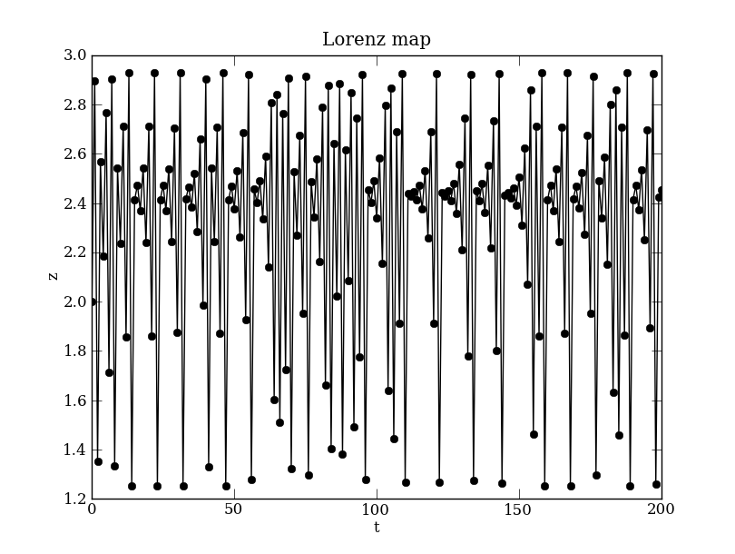
A 1D mapping can be derived from an approximation to the triple-zero unfolding of the Lorenz system of ODEs (e.g., see the original XPP tutorial example):
\( z(t+1) = a+b (z(t)-c)^2, \quad \) (Lor)
The system is specified using PyDSTool with
import PyDSTool as dst
from PyDSTool import args
import numpy as np
from matplotlib import pyplot as plt
DSargs = args(name='Lorenz map')
DSargs.varspecs = {'z': 'a+b*(z-c)**2', # note syntax for power
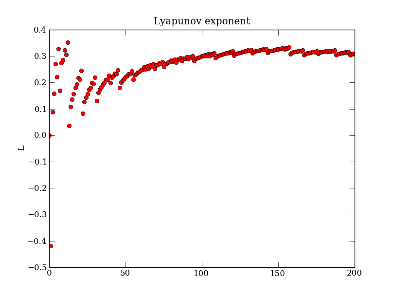
'zp': 'zp+log(abs(2*b*(z-c)))',
'L': 'zp/(t+1)'} # L is an auxiliary variable
DSargs.tdomain = [0, 200] # Default range of independent variable 't'
DSargs.pars = args(a=2.93,
b=-1.44,
c=1.85) # Using args() class to specify parameters with less syntax than a dictionary
DSargs.vars = ['z', 'zp'] # Implicitly, then, L will be an auxiliary variable
DSargs.ics = {'z': 2, 'zp': 0} # Initial conditions
DSargs.ttype = int # force independent variable type to be integer (discrete time)
Notice that the variable L is defined using t+1 because the discrete time begins at 0.
The solution of the discrete dynamical system Eq. (Lor) can be computed using a Generator mapping instance:
lmap = dst.Generator.MapSystem(DSargs)   # an instance of the 'Generator' class for maps.
traj = lmap.compute('test')              # compute a trajectory named 'test'
pts = traj.sample()                      # sample the points from the trajectory

# PyPlot commands
plt.figure(1)
plt.plot(pts['t'], pts['z'], 'ko-')
plt.title(lmap.name)
plt.xlabel('t')
plt.ylabel('z')

plt.figure(2)
plt.plot(pts['t'], pts['L'], 'ro')
plt.title('Lyapunov exponent')
plt.ylabel('L')
plt.xlabel('t')
plt.show()
Depending on your local configuration of the Matplotlib interactive mode, the last command plt.show() might not be necessary.