Site navigation:
We combine multiple tools in this example. We build the "two patch Rosenzweig-MacArthur predator-prey model" using PyDSTool's symbolic tools. For details of the mathematical model, see
"Predator migration in response to prey density: What are the consequences?"
by Y. Huang et al, J. Math Biol, Vol. 43, pp. 561-581, (2001)
The system of 4 ODEs is given by:
\( \left\{ \begin{align*} v1' &= v1*(1-v1/k) - v1*p1/(1+h*v1) \\ v2' &= v2*(1-v2/k) - v2*p2/(1+h*v2) \\ p1' &= -1*\mu*p1 + v1*p1/(1+h*v1) + D*(((1+\theta*h*v2)/(1+h*v2))*p2 - ((1+\theta*h*v1)/(1+h*v1))*p1) \\ p2' &= -1*\mu*p2 + v2*p2/(1+h*v2) + D*(((1+\theta*h*v1)/(1+h*v1))*p1 - ((1+\theta*h*v2)/(1+h*v2))*p2) \end{align*} \right. \qquad \qquad \) (PP)
In this example, we have an explicit relationship between the parameters that will yield a nontrivial equilibrium of Eq. (PP), which we denote (v1_0, v2_0, p1_0, p2_0). We will perform a continuation of the curve of equilibrium solutions as two parameters, D and k, are varied, using this starting point (see PyCont). To make it easy to specify the initial conditions of Eq. (PP) from the parameters, we take advantage of the symbolic classes in PyDSTool (see Symbolic). The system is specified using PyDSTool with
from PyDSTool import *

# Declare names and initial values for (symbolic) parameters
mu = Par(0.8, 'mu')
k = Par(7, 'k')
D = Par(0.5, 'D')
theta = Par(1, 'theta')
h = Par(0.5, 'h')

# Compute nontrivial boundary equilibrium initial condition from parameters (see reference for derivation)
v1_0 = mu*(2*D + mu) / (D*(1-h*mu-theta*h*mu) + mu*(1-h*mu))
v2_0 = 0.0
p1_0 = (1+h*v1_0)*(1-v1_0/k)
p2_0 = (D/(D+mu))*(1+theta*h*v1_0)*(1-v1_0/k)

# Declare symbolic variables
v1 = Var('v1')
v2 = Var('v2')
p1 = Var('p1')
p2 = Var('p2')

# Create Symbolic Quantity objects for definitions
v1rhs = v1*(1-v1/k) - v1*p1/(1+h*v1)
v2rhs = v2*(1-v2/k) - v2*p2/(1+h*v2)
p1rhs = -1*mu*p1 + v1*p1/(1+h*v1) + D*(((1+theta*h*v2)/(1+h*v2))*p2 - ((1+theta*h*v1)/(1+h*v1))*p1)
p2rhs = -1*mu*p2 + v2*p2/(1+h*v2) + D*(((1+theta*h*v1)/(1+h*v1))*p1 - ((1+theta*h*v2)/(1+h*v2))*p2)

# Build Generator
DSargs = args(name='PredatorPrey')
DSargs.pars = [mu, k, D, theta, h]
DSargs.varspecs = args(v1=v1rhs,
                       v2=v2rhs,
                       p1=p1rhs,
                       p2=p2rhs)
# Use eval method to get a float value from the symbolic definitions given in
# terms of parameter values
DSargs.ics = args(v1=v1_0.eval(), v2=v2_0, p1=p1_0.eval(), p2=p2_0.eval())
ode = Generator.Vode_ODEsystem(DSargs)
Notice that we do not provide string definitions of the ODE right-hand sides as we have before. The symbolic objects will be automatically converted when the Generator is initialized. To see the improved simplicity of this specification, compare it to the same model defined without symbolic objects in PyDSTool/tests/PyCont_PredPrey.py.
# Set up continuation class
PC = ContClass(ode)
PCargs = args(name='EQ1', type='EP-C')
PCargs.freepars = ['k']
PCargs.StepSize = 1e-2
PCargs.MaxNumPoints = 50
PCargs.MaxStepSize = 1e-1
PCargs.LocBifPoints = 'all'
PCargs.SaveEigen = True
PCargs.verbosity = 2
PC.newCurve(PCargs)
print 'Computing curve...'
start = clock()
PC['EQ1'].forward()
print 'done in %.3f seconds!' % (clock()-start)
PCargs.name = 'HO1'
PCargs.type = 'H-C2'
PCargs.initpoint = 'EQ1:H1'
PCargs.freepars = ['k','D']
PCargs.MaxNumPoints = 50
PCargs.MaxStepSize = 0.1
PCargs.LocBifPoints = ['ZH']
PCargs.SaveEigen = True
PC.newCurve(PCargs)
print 'Computing Hopf curve...'
start = clock()
PC['HO1'].forward()
print 'done in %.3f seconds!' % (clock()-start)
PCargs = args(name = 'FO1', type = 'LP-C')
PCargs.initpoint = 'HO1:ZH1'
PCargs.freepars = ['k','D']
PCargs.MaxNumPoints = 25
PCargs.MaxStepSize = 0.1
PCargs.LocBifPoints = 'all'
PCargs.SaveEigen = True
PC.newCurve(PCargs)
# Plot bifurcation diagram
PC.display(('k','D'), stability=True, figure=1)
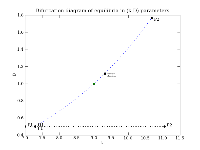
plt.title('Bifurcation diagram of equilibria in (k,D) parameters')
plt.show()
Depending on your local configuration of the Matplotlib interactive mode, the last command plt.show() might not be necessary. In the bifurcation diagram below, P1 and P2 refer to the start and end points of the continuation (one pair for forward, one for backward), and also correspond to labels in the solution pointset so that they may easily be extracted.
This is the terminal screen output from the script so far:
Computing curve...
Checking...
  |q| = 1.000000
  | - 1| =  8.67361737988e-19
  |Aq - iwq| = 0.000000
  |A*p + iwp| = 0.000000

H Point found
==========================
0 :
p2  =  0.568621188772
v1  =  2.48275862069
v2  =  0.0
p1  =  1.47841509081
k  =  7.29366287762

Eigenvalues =

     (0.000000,0.537392)
     (0.000000,-0.537392)
     (-1.467390,0.000000)
     (0.431379,0.000000)


w = 0.53739215535848206
l1 = -0.00018478829234509894

done in 0.451 seconds!
Computing Hopf curve...
ZH Point found
==========================
0 :
p2  =  1.00000000013
v1  =  3.45170289328
v2  =  -4.30952579626e-23
p1  =  1.71569147553
_k  =  0.220646854598
D  =  1.11780009629
k  =  9.314197349

Eigenvalues =

     (-2.541392,0.000000)
     (-0.000000,0.469731)
     (-0.000000,-0.469731)
     (-0.000000,0.000000)


done in 3.734 seconds!
This output shows that a codimension-2 Zero Hopf (ZH) point was found along the way (where a curve of fold points intersects), but we don't care about that in this example. See /tests/PyCont_PredPrey.py for more details of that.
Values of the two free parameters, D and k, are now found on the line of Hopf bifurcation points in the above figure, specified by k=9.0 (shown by the green dot). This value for k was chosen arbitrarily as an example. Because that value was not a point in the output of PyCont's continued solution, we use PyDSTool's Trajectory class to interpolate a value between the two nearest points.
# Create interpolatable curve from the pointset
hopfs_curve = pointset_to_traj(hopfs)
# Interpolate unstable Hopf equilibrium values of parameters/variables at k=9
Hpt = hopfs_curve(9.0)
Now we extract the state vector associated with that Hopf point, Hpt. Instead of needing to know the array indices associated with the variables and parameters stored in the pointset created by PyCont, PyDSTool lets us select them with a list of names. Instead of remembering those (e.g., if the system was much larger than 4D) we can simply provide the list stored in the Generator object. This is found in the vars attribute of its defining FuncSpec object (see FunctionalSpec). We find that the Hopf curve is unstable, so by slightly perturbing that state vector (for example in v2), we can integrate Eq. (PP) forward in time from that state vector as an initial condition, so that we should observe growing oscillations over a sufficiently long period of time. For a 3D projection of 3 out of the 4 variables, this appears to be the case.
# extract the variables defined for 'ode' Generator
Hics = Hpt[ode.funcspec.vars]
# perturb slightly off equilibrium
Hics['v2'] += 0.01

# extract the parameter value for D and indicate on bifurcation diagram
plt.plot(9.0, Hpt['D'], 'go')

ode.set(tdata=[0,100],
        pars={'k': 9.0, 'D': Hpt['D']},
        ics=Hics)
traj = ode.compute('test')
pts = traj.sample()

fig = plt.figure()
try:
    ax = fig.gca(projection='3d')
except ValueError:
    # pre-v1.0 version of Matplotlib
    ax = Axes3D(fig)
ax.plot(pts['v1'], pts['p1'], pts['p2'],
        label='Unstable periodic sol starting near eqm')

# to ensure your version accepts singleton points, enclose in extra brackets!
ax.plot(pts[[0]]['v1'], pts[[0]]['p1'], pts[[0]]['p2'], 'go', label='Initial condition')
ax.legend()
ax.set_xlabel('v1')
ax.set_ylabel('p1')
ax.set_zlabel('p2')
# 3D projection (v1,p1,p2) of unstable periodic sol. starting near eqm.
plt.draw()
plt.show()
The remaining screen output shows the results of finding and testing stability at the Hopf point at k=9.0.
k values found around 9.0 are 8.988, 9.071
Hopf point found for k = 8.988 is stable? No
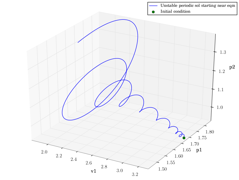
When you plot this graph, you can rotate it interactively. This example shows the use of the fledgling mplot3D package in Matplotlib. For more professional 3D graphics, you may wish to try MayaVi or others.